 (n) time in
the worst case--in practice, hashing performs extremely well. Under reasonable
assumptions, the expected time to search for an element in a hash table is
O(1).
(n) time in
the worst case--in practice, hashing performs extremely well. Under reasonable
assumptions, the expected time to search for an element in a hash table is
O(1).
A hash table is a generalization of the simpler notion of an ordinary array. Directly addressing into an ordinary array makes effective use of our ability to examine an arbitrary position in an array in O (1) time. Section 12.1 discusses direct addressing in more detail. Direct addressing is applicable when we can afford to allocate an array that has one position for every possible key.
When the number of keys actually stored is small relative to the total number of possible keys, hash tables become an effective alternative to directly addressing an array, since a hash table typically uses an array of size proportional to the number of keys actually stored. Instead of using the key as an array index directly, the array index is computed from the key. Section 12.2 presents the main ideas, and Section 12.3 describes how array indices can be computed from keys using hash functions. Several variations on the basic theme are presented and analyzed; the "bottom line" is that hashing is an extremely effective and practical technique: the basic dictionary operations require only O (1) time on the average.
12.1 Direct-address tables
Direct addressing is a simple technique that works well when the
universe U of keys is reasonably small. Suppose that an application needs
a dynamic set in which each element has a key drawn from the universe U =
{0,1, . . . , m - 1}, where m is not too large. We shall assume that no
two elements have the same key.
To
represent the dynamic set, we use an array, or direct-address
table, T [0 . . m - 1], in which each position, or
slot, corresponds to a key in the universe U. Figure 12.1
illustrates the approach; slot k points to an element in the set with key
k. If the set contains no element with key k, then
T[k] = NIL.
The dictionary operations are trivial to implement.
Each of these operations is fast: only O(1) time is required.
For some applications, the elements in the dynamic set can be stored in the
direct-address table itself. That is, rather than storing an element's key and satellite data in an object
external to the direct-address table, with a pointer from a slot in the table to
the object, we can store the object in the slot itself, thus saving space.
Moreover, it is often unnecessary to store the key field of the object, since if
we have the index of an object in the table, we have its key. If keys are not
stored, however, we must have some way to tell if the slot is empty.
12.1-1
Consider a dynamic set S that is represented by a direct-address table
T of length m. Describe a procedure that finds the maximum element
of S. What is the worst-case performance of your procedure?
12.1-2
A bit vector is simply an
array of bits (0's and 1's). A bit vector of length m takes
much less space than an array of m pointers. Describe how to use a bit
vector to represent a dynamic set of distinct elements with no satellite data.
Dictionary operations should run in O(1) time.
12.1-3
Suggest how to implement a direct-address table in which the keys of stored
elements do not need to be distinct and the elements can have satellite data.
All three dictionary operations (INSERT,
DELETE, and SEARCH) should run in O(1) time. (Don't forget that DELETE takes as an argument a pointer to an
object to be deleted, not a key.)
12.1-4
We wish to implement a dictionary by using direct addressing on a huge
array. At the start, the array entries may contain garbage, and initializing
the entire array is impractical because of its size. Describe a scheme for
implementing a direct-address dictionary on a huge array. Each stored object
should use O(1) space; the operations SEARCH, INSERT, and DELETE should take O(1) time each; and
the initialization of the data structure should take O(1) time.
(Hint: Use an additional stack, whose size is the number of keys actually
stored in the dictionary, to help determine whether a given entry in the huge
array is valid or not.)
The difficulty with
direct addressing is obvious: if the universe U is large, storing a table
T of size |U| may be impractical, or even impossible, given the
memory available on a typical computer. Furthermore, the set K of keys
actually stored may be so small relative to U that most of the
space allocated for T would be wasted.
When the set K of keys stored in a dictionary is much smaller than the
universe U of all possible keys, a hash table requires much less storage
than a direct-address table. Specifically, the storage requirements can be
reduced to
With direct addressing, an element with key k is
stored in slot k. With hashing, this element is stored in slot
h(k); that is, a hash function h is used to
compute the slot from the key k. Here h maps the universe U
of keys into the slots of a hash table T[0 . . m -
1]:
We say that an element with key k
hashes to slot h(k); we also say that h(k) is the
hash value of key k. Figure 12.2 illustrates the basic
idea. The point of the hash function is to reduce the range of array indices
that need to be handled. Instead of |U| values, we need to handle only
m values. Storage requirements are correspondingly reduced.
The fly in the ointment of this beautiful idea is that two
keys may hash to the same slot--a collision. Fortunately, there
are effective techniques for resolving the conflict created by collisions.
Of course, the ideal solution would be to avoid collisions altogether. We
might try to achieve this goal by choosing a suitable hash function h.
One idea is to make h appear to be "random," thus avoiding collisions or
at least minimizing their number. The very term "to hash," evoking images of
random mixing and chopping, captures the spirit of this approach. (Of course, a
hash function h must be deterministic in that a given input k
should always produce the same output h(k).) Since |U| >
m, however, there must be two keys that have the same hash value;
avoiding collisions altogether is therefore impossible. Thus, while a
well-designed, "random"- looking hash function can minimize the number of
collisions, we still need a method for resolving the collisions that do occur.
The remainder of this section presents the simplest collision resolution
technique, called chaining. Section 12.4 introduces an alternative method for
resolving collisions, called open addressing.
In
chaining, we put all the elements that hash to the same slot in a
linked list, as shown in Figure 12.3. Slot j contains a pointer to the
head of the list of all stored elements that hash to j; if there are no
such elements, slot j contains NIL.
The dictionary operations on a hash table T are easy to implement when
collisions are resolved by chaining.
The worst-case running time for insertion is O(1). For searching, the
worst-case running time is proportional to the length of the list; we shall
analyze this more closely below. Deletion of an element x can be
accomplished in O(1) time if the lists are doubly linked. (If the lists
are singly linked, we must first find x in the list
T[h(key[x])], so that the next link of
x's predecessor can be properly set to splice x out; in this case,
deletion and searching have essentially the same running time.)
How well does hashing with chaining perform? In particular,
how long does it take to search for an element with a given key?
Given a hash table T with m slots that stores
n elements, we define the load factor The worst-case behavior of hashing with chaining is terrible: all n
keys hash to the same slot, creating a list of length n. The worst-case
time for searching is thus The average performance of hashing depends on how well the
hash function h distributes the set of keys to be stored among the
m slots, on the average. Section 12.3 discusses these issues, but for now
we shall assume that any given element is equally likely to hash into any of the
m slots, independently of where any other element has hashed to. We call
this the assumption of simple uniform hashing.
We assume that the hash value h(k) can be computed in
O(1) time, so that the time required to search for an element with key
k depends linearly on the length of the list
T[h(k)]. Setting aside the O(1) time required to
compute the hash function and access slot h(k), let us consider
the expected number of elements examined by the search algorithm, that is, the
number of elements in the list T[h(k)] that are checked to
see if their keys are equal to k. We shall consider two cases. In the
first, the search is unsuccessful: no element in the table has key k. In
the second, the search successfully finds an element with key k.
Theorem 12.1
In a hash table in which collisions are resolved by chaining, an unsuccessful
search takes time Proof Under the assumption of simple uniform hashing, any key
k is equally likely to hash to any of the m slots. The average
time to search unsuccessfully for a key k is thus the average time to
search to the end of one of the m lists. The average length of such a
list is the load factor Theorem 12.2
In a hash table in which collisions are resolved by
chaining, a successful search takes time Proof We assume that the key being searched for is equally
likely to be any of the n keys stored in the table. We also assume that
the CHAINED-HASH-INSERT procedure
inserts a new element at the end of the list instead of the front. (By Exercise
12.2-3, the average successful search time is the same whether new elements are
inserted at the front of the list or at the end.) The expected number of
elements examined during a successful search is 1 more than the number of
elements examined when the sought-for element was inserted (since every new
element goes at the end of the list). To find the expected number of elements
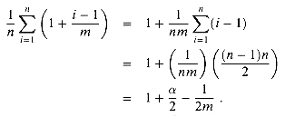
examined, we therefore take the average, over the n items in the table,
of 1 plus the expected length of the list to which the ith element is
added. The expected length of that list is (i- 1)/m, and so the
expected number of elements examined in a successful search is
Thus, the total time required for a successful search (including the time for
computing the hash function) is What does this analysis mean? If the number of hash-table slots is at least
proportional to the number of elements in the table, we have n =
O(m) and, consequently,
12.2-1
Suppose we use a random hash function h to hash n distinct keys
into an array T of length m. What is the expected number of
collisions? More precisely, what is the expected cardinality of
{(x,y): h(x) = h(y)}?
12.2-2
Demonstrate the insertion of the keys 5, 28, 19, 15, 20, 33, 12, 17, 10 into
a hash table with collisions resolved by chaining. Let the table have 9 slots,
and let the hash function be h(k) = k mod 9.
12.2-3
Argue that the expected time for a successful search with chaining is the
same whether new elements are inserted at the front or at the end of a list.
(Hint: Show that the expected successful search time is the same for
any two orderings of any list.)
12.2-4
Professor Marley hypothesizes that substantial performance gains can be
obtained if we modify the chaining scheme so that each list is kept in sorted
order. How does the professor's modification affect the running time for
successful searches, unsuccessful searches, insertions, and deletions?
12.2-5
Suggest how storage for elements can be allocated and
deallocated within the hash table itself by linking all unused slots into a free
list. Assume that one slot can store a flag and either one element plus a
pointer or two pointers. All dictionary and free-list operations should run in
O(l) expected time. Does the free list need to be doubly linked, or does
a singly linked free list suffice?
12.2-6
Show that if |U| > nm, there is a subset of U of size
n consisting of keys that all hash to the same slot, so that the
worst-case searching time for hashing with chaining is
In this section, we discuss some issues regarding the
design of good hash functions and then present three schemes for their creation:
hashing by division, hashing by multiplication, and universal hashing.
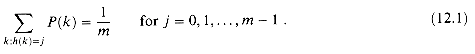
A good hash function satisfies (approximately) the assumption of simple
uniform hashing: each key is equally likely to hash to any of the m
slots. More formally, let us assume that each key is drawn independently from
U according to a probability distribution P; that is, P(k)
is the probability that k is drawn. Then the assumption of simple uniform
hashing is that
Unfortunately, it is generally not possible to check this condition, since
P is usually unknown.
Sometimes (rarely) we do know the distribution P. For example, suppose
the keys are known to be random real numbers k independently and
uniformly distributed in the range 0 can be shown to satisfy equation (12.1).
In practice, heuristic techniques can be used to create a
hash function that is likely to perform well. Qualitative information about
P is sometimes useful in this design process. For example, consider a
compiler's symbol table, in which the keys are arbitrary character strings
representing identifiers in a program. It is common for closely related symbols,
such as pt and pts, to occur in the same program. A good hash function would
minimize the chance that such variants hash to the same slot.
A common approach is to derive the hash value in a way that is expected to be
independent of any patterns that might exist in the data. For example, the
"division method" (discussed further below) computes the hash value as the
remainder when the key is divided by a specified prime number. Unless that prime
is somehow related to patterns in the probability distribution P, this
method gives good results.
Finally, we note that some applications of hash functions might require
stronger properties than are provided by simple uniform hashing. For example, we
might want keys that are "close" in some sense to yield hash values that are far
apart. (This property is especially desirable when we are using linear probing,
defined in Section 12.4.)
Most hash functions assume that the universe of keys is the set N =
{0,1,2, . . .} of natural numbers. Thus, if the keys are not natural numbers, a
way must be found to interpret them as natural numbers. For example, a key that
is a character string can be interpreted as an integer expressed in suitable
radix notation. Thus, the identifier pt
might be interpreted as the pair of decimal integers (112,116), since p = 112 and t = 116 in the ASCII character set; then, expressed as a radix-128
integer, pt becomes (112
In the division method for
creating hash functions, we map a key k into one of m slots by
taking the remainder of k divided by m. That is, the hash function
is
For example, if the hash table has size m = 12 and the key is k
= 100, then h(k) = 4. Since it requires only a single division operation,
hashing by division is quite fast.
When using the division method, we usually avoid certain values of m.
For example, m should not be a power of 2, since if m =
2p, then h(k) is just the p lowest-order bits of
k. Unless it is known a priori that the probability distribution on keys
makes all low-order p-bit patterns equally likely, it is better to make
the hash function depend on all the bits of the key. Powers of 10 should be
avoided if the application deals with decimal numbers as keys, since then the
hash function does not depend on all the decimal digits of k. Finally, it
can be shown that when m = 2p - 1 and k is a
character string interpreted in radix 2p, two strings that are
identical except for a transposition of two adjacent characters will hash to the
same value.
Good values for m are primes not too close to exact powers of 2. For
example, suppose we wish to allocate a hash table, with collisions resolved by
chaining, to hold roughly n = 2000 character strings, where a character
has 8 bits. We don't mind examining an average of 3 elements in an unsuccessful
search, so we allocate a hash table of size m = 701. The number 701 is
chosen because it is a prime near As a precautionary measure, we could check how evenly this hash function
distributes sets of keys among the slots, where the keys are chosen from "real"
data.
The multiplication method
for creating hash functions operates in two steps. First, we multiply the key
k by a constant A in the range 0 < A < 1 and extract
the fractional part of kA. Then, we multiply this value by m and
take the floor of the result. In short, the hash function is
where "k A mod 1" means the fractional part of kA, that is,
kA - An advantage of the multiplication method is that the value of m is
not critical. We typically choose it to be a power of 2--m =
2p for someinteger p--since we can then easily
implement the function on most computers as follows. Suppose that the word size
of the machine is w bits and that k fits into a single word.
Referring to Figure 12.4, we first multiply k by the w-bit integer
Although this method works with any value of the constant A, it works
better with some values than with others. The optimal choice depends on the
characteristics of the data being hashed. Knuth [123] discusses the choice of
A in some detail and suggests that
is likely to work reasonably well.
As an example, if we have k = 123456, m = 10000, and A
as in equation (12.2), then
If a
malicious adversary chooses the keys to be hashed, then he can choose n
keys that all hash to the same slot, yielding an average retrieval time of The main idea behind universal hashing is to select the
hash function at random at run time from a carefully designed class of
functions. As in the case of quicksort, randomization guarantees that no single
input will always evoke worst-case behavior. Because of the randomization, the
algorithm can behave differently on each execution, even for the same input.
This approach guarantees good average-case performance, no matter what keys are
provided as input. Returning to the example of a compiler's symbol table, we
find that the programmer's choice of
identifiers cannot now cause consistently poor hashing performance. Poor
performance occurs only if the compiler chooses a random hash function that
causes the set of identifiers to hash poorly, but the probability of this
occurring is small and is the same for any set of identifiers of the same size.
Let The following theorem shows that a universal class of hash functions gives
good average-case behavior.
Theorem 12.3
If h is chosen from a universal collection of hash functions and is
used to hash n keys into a table of size m, where n Proof For each pair y, z of distinct keys, let
cyz be a random variable that is 1 if h(y) =
h(z) (i.e., if y and z collide using h) and 0
otherwise. Since, by definition, a single pair of keys collides with probability
1/m, we have
Let Cx be the total number of collisions involving key
x in a hash table T of size m containing n keys.
Equation (6.24) gives
Since n But how easy is it to design a universal class of hash functions? It is quite
easy, as a little number theory will help us prove. Let us choose our table size
m to be prime (as in the division method). We decompose a key x
into r+ 1 bytes (i.e., characters, or fixed-width binary substrings), so
that x =
With this definition,
has mr+1 members.
Theorem 12.4
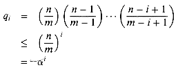
The class Proof Consider any pair of distinct keys x, y. Assume
that x0 To see this property, note that since m is prime,
the nonzero quantity x0 - y0 has a
multiplicative inverse modulo m, and thus there is a unique solution for
a0 modulo m. (See Section 33.4.) Therefore, each pair
of keys x and y collides for exactly mr values
of a, since they collide exactly once for each possible value of
12.3-1
Suppose we wish to search a linked list of length n,
where each element contains a key k along with a hash value
h(k). Each key is a long character string. How might we take
advantage of the hash values when searching the list for an element with a given
key?
12.3-2
Suppose a string of r characters is hashed into m slots by
treating it as a radix-128 number and then using the division method. The number
m is easily represented as a 32-bit computer word, but the string of
r characters, treated as a radix-128 number, takes many words. How can we
apply the division method to compute the hash value of the character string
without using more than a constant number of words of storage outside the string
itself?
12.3-3
Consider a version of the division method in which h(k) =
k mod m, where m = 2p - I and k is a
character string interpreted in radix 2p. Show that if string
x can be derived from string y by permuting its characters, then
x and y hash to the same value. Give an example of an application
in which this property would be undesirable in a hash function.
12.3-4
Consider a hash table of size m = 1000 and the hash function
h(k) = 12.3-5
Show that if we restrict each component ai of a in
equation (12.3) to be nonzero, then the set
In open
addressing, all elements are stored in the hash table itself. That is,
each table entry contains either an element of the dynamic set or NIL. When searching for an element, we
systematically examine table slots until the desired element is found or it is
clear that the element is not in the table. There are no lists and no elements
stored outside the table, as there are in chaining. Thus, in open addressing,
the hash table can "fill up" so that no further insertions can be made; the load
factor Of course, we could store the linked lists for chaining inside the hash
table, in the otherwise unused hash-table slots (see Exercise 12.2-5), but the
advantage of open addressing is that it avoids pointers altogether. Instead of
following pointers, we compute the sequence of slots to be examined. The
extra memory freed by not storing pointers provides the hash table with a larger
number of slots for the same amount of memory, potentially yielding fewer
collisions and faster retrieval.
To perform insertion
using open addressing, we successively examine, or probe, the hash
table until we find an empty slot in which to put the key. Instead of being
fixed in the order 0, 1, . . . , m - 1 (which requires With open addressing, we require that for every key k, the probe
sequence
be a permutation of The algorithm for searching for key k probes the same sequence of
slots that the insertion algorithm examined when key k was inserted.
Therefore, the search can terminate (unsuccessfully) when it finds an empty
slot, since k would have been inserted there and not later in its probe
sequence. (Note that this argument assumes that keys are not deleted from the
hash table.) The procedure HASH-SEARCH takes as input a hash table T and
a key k, returning j if slot j is found to contain key
k, or NIL if key k is
not present in table T.
Deletion from an open-address hash table is difficult. When
we delete a key from slot i, we cannot simply mark that slot as empty by
storing NIL in it. Doing so might make it
impossible to retrieve any key k during whose insertion we had probed
slot i and found it occupied. One solution is to mark the slot by storing
in it the special value DELETED instead
of NIL. We would then modify the
procedure HASH-SEARCH so that it keeps on looking when it sees the value DELETED, while HASH-INSERT would treat
such a slot as if it were empty so that a new key can be inserted. When we do
this, though, the search times are no longer dependent on the load factor In our analysis, we make the assumption of uniform
hashing: we assume that each key considered is equally likely to have
any of the m! permutations of {0, 1, . . . , m - 1} as its probe
sequence. Uniform hashing generalizes the notion of simple uniform hashing
defined earlier to the situation in which the hash function produces not just a
single number, but a whole probe sequence. True uniform hashing is difficult to
implement, however, and in practice suitable approximations (such as double
hashing, defined below) are used.
Three techniques are commonly used to compute the probe sequences required
for open addressing: linear probing, quadratic probing, and double hashing.
These techniques all guarantee that
Given an ordinary hash function
h': U for i = 0,1,...,m - 1. Given key k, the first slot
probed is T[h'(k)]. We next probe slot
T[h'(k) + 1], and so on up to slot T[m - 1].
Then we wrap around to slots T[0], T[1], . . . , until we finally
probe slot T[h'(k) - 1]. Since the initial probe position
determines the entire probe sequence, only m distinct probe sequences are
used with linear probing.
Linear probing is easy to implement, but
it suffers from a problem known as primary clustering. Long runs
of occupied slots build up, increasing the average search time. For example, if
we have n = m/2 keys in the table, where every even-indexed slot
is occupied and every odd-indexed slot is empty, then the average unsuccessful
search takes 1.5 probes. If the first n = m/2 locations are the
ones occupied, however, the average number of probes increases to about
n/4 = m/8. Clusters are likely to arise, since if an empty slot is
preceded by i full slots, then the probability that the empty slot is the
next one filled is (i + 1)/m, compared with a probability of
1/m if the preceding slot was empty. Thus, runs of occupied slots tend to
get longer, and linear probing is not a very good approximation to uniform
hashing.
Quadratic
probing uses a hash function of the form
where (as in linear probing) h' is an auxiliary hash function,
c1 and c2
Double hashing is one of the best methods
available for open addressing because the permutations produced have many of the
characteristics of randomly chosen permutations. Double hashing
uses a hash function of the form
where h1 and h2 are auxiliary hash
functions. The initial position probed is T[h1
(k)]; successive probe positions are offset from previous positions by
the amount h2(k), modulo m. Thus, unlike the
case of linear or quadratic probing, the probe sequence here depends in two ways
upon the key k, since the initial probe position, the offset, or both,
may vary. Figure 12.5 gives an example of insertion by double hashing.
The value h2(k) must be relatively prime to the
hash-table size m for the entire hash table to be searched. Otherwise, if
m and h2(k) have greatest common divisor
d > 1 for some key k, then a search for key k would
examine only (1/d)th of the hash table. (See Chapter 33.) A convenient
way to ensure this condition is to let m be a power of 2 and to design
h2 so that it always produces an odd number. Another way is to
let m be prime and to design h2 so that it always
returns a positive integer less than m. For example, we could choose
m prime and let
where m' is chosen to be slightly less than m (say, m -
1 or m - 2). For example, if k = 123456 and m = 701, we
have h1(k) = 80 and h2(k) =
257, so the first probe is to position 80, and then every 257th slot (modulo
m) is examined until the key is found or every slot is examined.
Double hashing represents an improvement over linear or quadratic probing in
that
Our analysis of open addressing, like our analysis of
chaining, is expressed in terms of the load factor We assume that uniform hashing is used. In this idealized scheme, the probe
sequence We now analyze the expected number of probes for hashing with open addressing
under the assumption of uniform hashing, beginning with an analysis of the
number of probes made in an unsuccessful search.
Theorem 12.5
Given an open-address hash table with load factor Proof In an unsuccessful search, every probe but the last
accesses an occupied slot that does not contain the desired key, and the last
slot probed is empty. Let us define
pi = Pr {exactly i probes access occupied slots}
for i = 0, 1, 2, . . . . For i > n, we have
pi = 0, since we can find at most n slots already
occupied. Thus, the expected number of probes is
To evaluate equation (12.6), we define
qi = Pr {at least i probes access occupied slots}
for i = 0, 1, 2, . . . . We can then use identity (6.28):
What is the value of qi for i With uniform hashing, a second probe, if necessary, is to one of the
remaining m - 1 unprobed slots, n - 1 of which are occupied. We
make a second probe only if the first probe accesses an occupied slot; thus,
In general, the ith probe is made only if the first i - 1
probes access occupied slots, and the slot probed is equally likely to be any of
the remaining m - i + 1 slots, n - i + 1 of which
are occupied. Thus,
for i = 1, 2, . . . , n, since (n - j) /
(m - j) We are now ready to evaluate equation (12.6). Given the assumption that
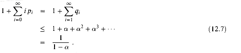
Equation (12.7) has an intuitive interpretation: one probe is always made,
with probability approximately If Theorem 12.5 gives us the performance of the HASH-INSERT procedure
almost immediately.
Corollary 12.6
Inserting an element into an open-address hash table with load factor Proof An element is inserted only if there is room in the
table, and thus Computing the expected number of probes for a successful search requires a
little more work.
Theorem 12.7
Given an open-address hash table with load factor assuming uniform hashing and assuming that each key in the table is equally
likely to be searched for.
Proof A search for a key k follows the same probe
sequence as was followed when the element with key k was inserted. By
Corollary 12.6, if k was the (i + 1)st key inserted into the hash
table, the expected number of probes made in a search for k is at most 1
/ (1 - i/m) = m/(m - i). Averaging over all n
keys in the hash table gives us the average number of probes in a successful
search:
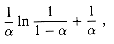
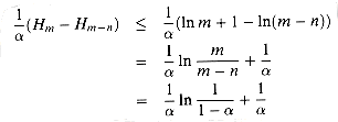
where Hi = for a bound on the expected number of probes in a successful search.
If the hash table is half full, the expected number of probes is less than
3.387. If the hash table is 90 percent full, the expected number of probes is
less than 3.670.
12.4-1
Consider inserting the keys 10, 22, 31, 4, 15, 28, 17, 88,
59 into a hash table of length m = 11 using open addressing with the
primary hash function h'(k) = k mod m. Illustrate
the result of inserting these keys using linear probing, using quadratic probing
with c1 = 1 and c2 = 3, and using double
hashing with h2(k) = 1 + (k mod (m - 1)).
12.4-2
Write pseudocode for
HASH-DELETE as outlined in the text, and modify HASH-INSERT and HASH-SEARCH to incorporate the special value DELETED.
12.4-3
Suppose that we use double hashing to resolve collisions;
that is, we use the hash function h(k, i) =
(h1(k) + ih2(k)) mod m.
Show that the probe sequence 12.4-4
Consider an open-address hash table with uniform hashing and a load factor
12.4-5
Suppose that we insert n keys into a hash table of size m using
open addressing and uniform hashing. Let p(n, m) be the
probability that no collisions occur. Show that p(n, m)
12.4-6
The bound on the harmonic series can be
improved to
where 12.4-7
Consider an open-address hash table with a load factor
12-1 Longest-probe bound for hashing
A hash table of size m is used to
store n items, with n a. Assuming uniform hashing, show that for i = 1, 2, . .
. , n, the probability that the ith insertion requires strictly
more than k probes is at most 2-k.
b. Show that for i = 1, 2, . . ., n, the
probability that the ith insertion requires more than 2 lg n
probes is at most 1/n2.
Let the random variable Xi denote the number of probes
required by the ith insertion. You have shown in part (b) that
Pr{Xi >2 1g n} c. Show that Pr{X > 2 1g n} d. Show that the expected length of the longest probe sequence
is E[X] = O(lg n)
12-2 Searching a static set
You
are asked to implement a dynamic set of n elements in which the keys are
numbers. The set is static (no INSERT or
DELETE operations), and the only
operation required is SEARCH. You are
given an arbitrary amount of time to preprocess the n elements so that
SEARCH operations run quickly.
a. Show that SEARCH can
be implemented in O(1g n) worst-case time using no extra storage
beyond what is needed to store the elements of the set themselves.
b. Consider implementing the set by open-address hashing on
m slots, and assume uniform hashing. What is the minimum amount of extra
storage m - n required to make the average performance of an
unsuccessful SEARCH operation be at least
as good as the bound in part (a)? Your answer should be an asymptotic bound on
m - n in terms of n.
12-3 Slot-size bound for chaining
Suppose that we have a
hash table with n slots, with collisions resolved by chaining, and
suppose that n keys are inserted into the table. Each key is equally
likely to be hashed to each slot. Let M be the maximum number of keys in
any slot after all the keys have been inserted. Your mission is to prove an
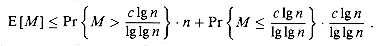
O(1g n/1g 1g n) upper bound on E[M], the
expected value of M.
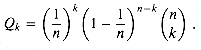
a. Argue that the probability Qk that
k keys hash to a particular slot is given by
b. Let Pk be the probability that M =
k, that is, the probability that the slot containing the most keys
contains k keys. Show that Pk c. Use Stirling's approximation, equation (2.1l), to show that
Qk < ek/kk.
d. Show that there exists a constant c > 1 such that
Qk0 <
1/n3 for k0 = c lg n/lg lg
n. Conclude that Pk0 < 1/n2 for k0 =
c lg n/lg lg n.
e. Argue that
Conclude that E [M] = O(lg n/1g 1g n).
12-4 Quadratic probing
Suppose that we are given a key k
to search for in a hash table with positions 0, 1, . . . , m - 1, and
suppose that we have a hash function h mapping the key space into the set
{0, 1, . . . , m - 1}. The search scheme is as follows.
1. Compute the value i 2. Probe in position i for the desired key k. If you find it,
or if this position is empty, terminate the search.
3. Set j Assume that m is a power of 2.
a. Show that this scheme is an instance of the general
"quadratic probing" scheme by exhibiting the appropriate constants
c1 and c2 for equation (12.5).
b. Prove that this algorithm examines every table position in
the worst case.
12-5 k-universal hashing
Let a. Show that if b. Show that the class c. Show that if we modify the definition of then
Knuth [123] and Gonnet [90] are excellent references for the analysis of
hashing algorithms. Knuth credits H. P. Luhn (1953) for inventing hash tables,
along with the chaining method for resolving collisions. At about the same time,
G. M. Amdahl originated the idea of open addressing.
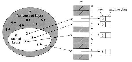
Figure 12.1 Implementing a dynamic set by a direct-address
table T. Each key in the universe U = {0,1, . . . , 9} corresponds to an index
in the table. The set K = {2, 3, 5, 8} of actual keys determines the slots in
the table that contain pointers to elements. The other slots, heavily shaded,
contain NIL.
DIRECT-ADDRESS-SEARCH(T,k)
return T[k]
DIRECT-ADDRESS-INSERT(T,x)
T[key[x]]
 x
xDIRECT-ADDRESS-DELETE(T,x)
T[key[x]]
NILExercises
12.2 Hash tables
(|K|),
even though searching for an element in the hash table still requires only
O(1) time. (The only catch is that this bound is for the average
time, whereas for direct addressing it holds for the worst-case
time.)
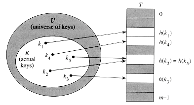
Figure 12.2 Using a hash function h to map keys to
hash-table slots. Keys k2 and
k5 map to the same slot, so they
collide.
h: U
 {0,1, . . . , m - 1} .
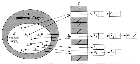
Figure 12.3 Collision resolution by chaining. Each
hash-table slot T[j] contains a linked list of all the keys whose hash value is
j. For example, h(k1) =
h(k4) and h(k5) = h(k2) = h(k7).
Collision resolution by chaining
CHAINED-HASH-INSERT(T,x)
insert x at the head of list T[h(key[x])]
CHAINED-HASH-SEARCH(T,k)
search for an element with key k in list T[h(k)]
CHAINED-HASH-DELETE(T,x)
delete x from the list T[h(key[x])]
Analysis of hashing with chaining
 for T as n/m, that
is, the average number of elements stored in a chain. Our analysis will be in
terms of ; that is, we imagine
staying fixed as n and
m go to infinity. (Note that can be less than, equal to, or
greater than l .)
(n) plus the time to compute
the hash function--no better than if we used one linked list for all the
elements. Clearly, hash tables are not used for their worst-case performance.
(1 + ), on the average, under the
assumption of simple uniform hashing.
=
n/m. Thus, the expected number of elements examined in an unsuccessful
search is , and the total time
required (including the time for computing h(k)) is (1 + ).
(1 +), on the average, under the
assumption of simple uniform hashing.
for T as n/m, that
is, the average number of elements stored in a chain. Our analysis will be in
terms of ; that is, we imagine
staying fixed as n and
m go to infinity. (Note that can be less than, equal to, or
greater than l .)
(n) plus the time to compute
the hash function--no better than if we used one linked list for all the
elements. Clearly, hash tables are not used for their worst-case performance.
(1 + ), on the average, under the
assumption of simple uniform hashing.
=
n/m. Thus, the expected number of elements examined in an unsuccessful
search is , and the total time
required (including the time for computing h(k)) is (1 + ).
(1 +), on the average, under the
assumption of simple uniform hashing.
 (2 + /2 - 1/2m) = (1 + ).
= n/m =
O(m)/m = O(1). Thus, searching takes constant time
on average. Since insertion takes O( l ) worst-case time (see Exercise
12.2-3), and deletion takes O(l) worst-case time when the lists are
doubly linked, all dictionary operations can be supported in O( l ) time
on average.
(2 + /2 - 1/2m) = (1 + ).
= n/m =
O(m)/m = O(1). Thus, searching takes constant time
on average. Since insertion takes O( l ) worst-case time (see Exercise
12.2-3), and deletion takes O(l) worst-case time when the lists are
doubly linked, all dictionary operations can be supported in O( l ) time
on average.
Exercises
(n).
12.3 Hash functions
What makes a good hash function?
(12.1)
 k < 1. In this case, the
hash function
k < 1. In this case, the
hash function
h(k) =
 km
km
Interpreting keys as natural numbers
 128) + 116 = 14452. It is usually
straightforward in any given application to devise some such simple method for
interpreting each key as a (possibly large) natural number. In what follows, we
shall assume that the keys are natural numbers.
128) + 116 = 14452. It is usually
straightforward in any given application to devise some such simple method for
interpreting each key as a (possibly large) natural number. In what follows, we
shall assume that the keys are natural numbers.
12.3.1 The division method
h(k) = k mod m .
= 2000/3 but not near any power of
2. Treating each key k as an integer, our hash function would be
h(k) = k mod 701 .
12.3.2 The multiplication method
h(k) =
m (k A mod 1) ,kA.
A 2w. The result is a 2w-bit
value r1 2w + r0, where
r1 is the high-order word of the product and
r0 is the low-order word of the product. The desired
p-bit hash value consists of the p most significant bits of
r0.
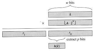
Figure 12.4 The multiplication method of hashing. The
w-bit representation of the key k is multiplied by the w-bit value
A.2w, where 0 < A < 1 is a suitable constant. The p
highest-order bits of the lower w-bit half of the product form the desired hash
value h(k).
(12.2)
h(k) =
10000 (123456 0.61803 . . . mod 1)=
10000 (76300.0041151. . . mod 1)=
10000 0.0041151 . . .=
41.151 . . .= 41 .
12.3.3 Universal hashing
(n). Any fixed hash function
is vulnerable to this sort of worst-case behavior; the only effective way to
improve the situation is to choose the hash function randomly in a way
that is independent of the keys that are actually going to be stored.
This approach, called universal hashing, yields good performance
on the average, no matter what keys are chosen by the adversary.
 be a finite collection of
hash functions that map a given universe U of keys into the range {0,1, .
. . , m - 1}. Such a collection is said to be universal if
for each pair of distinct keys x,y
be a finite collection of
hash functions that map a given universe U of keys into the range {0,1, .
. . , m - 1}. Such a collection is said to be universal if
for each pair of distinct keys x,y  U, the number of hash functions
 for which h(x) =
h(y) is precisely
for which h(x) =
h(y) is precisely  .
In other words, with a hash function randomly chosen from
.
In other words, with a hash function randomly chosen from  , the chance of a collision between
x and y when x
, the chance of a collision between
x and y when x  y is exactly 1/m, which is
exactly the chance of a collision if h(x) and h(y)
are randomly chosen from the set {0,1, . . . , m - 1}.
m, the expected number of
collisions involving a particular key x is less than 1.
y is exactly 1/m, which is
exactly the chance of a collision if h(x) and h(y)
are randomly chosen from the set {0,1, . . . , m - 1}.
m, the expected number of
collisions involving a particular key x is less than 1.
E[cyz] = 1/m .
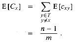 m, we
have E [Cx] < 1.
m, we
have E [Cx] < 1.
 x0,
x1,. . . , xr
x0,
x1,. . . , xr ; the only requirement is that the
maximum value of a byte should be less than m. Let a = a0,
a1, . . . , ar denote a sequence of r + 1
elements chosen randomly from the set {0,1, . . . , m - 1}. We define a
corresponding hash function
; the only requirement is that the
maximum value of a byte should be less than m. Let a = a0,
a1, . . . , ar denote a sequence of r + 1
elements chosen randomly from the set {0,1, . . . , m - 1}. We define a
corresponding hash function  :
:

(12.3)

(12.4)
 defined by
equations (12.3) and (12.4) is a universal class of hash functions.
y0. (A similar argument can be made for a difference in any
other byte position.) For any fixed values of a1,
a2, . . . , ar, there is exactly one value
of a0 that satisfies the equation h(x) =
h(y); this a0 is the solution to
defined by
equations (12.3) and (12.4) is a universal class of hash functions.
y0. (A similar argument can be made for a difference in any
other byte position.) For any fixed values of a1,
a2, . . . , ar, there is exactly one value
of a0 that satisfies the equation h(x) =
h(y); this a0 is the solution to
 al,
a2, . . ., ar (i.e., for the unique value
of a0 noted above).
Since there are mr+l possible values for the sequence a, keys
x and y collide with probability exactly
mr/mr+1 = 1/m. Therefore,
al,
a2, . . ., ar (i.e., for the unique value
of a0 noted above).
Since there are mr+l possible values for the sequence a, keys
x and y collide with probability exactly
mr/mr+1 = 1/m. Therefore,  is universal.
Exercises
m (k A mod
1) for A =  . Compute the locations to which the
keys 61, 62, 63, 64, and 65 are mapped.
. Compute the locations to which the
keys 61, 62, 63, 64, and 65 are mapped.
 as defined in equation (12.4) is not
universal. (Hint: Consider the keys x = 0 and y = 1.)
as defined in equation (12.4) is not
universal. (Hint: Consider the keys x = 0 and y = 1.)
12.4 Open addressing
can never exceed 1.
(n) search time), the sequence
of positions probed depends upon the key being inserted. To determine
which slots to probe, we extend the hash function to include the probe number
(starting from 0) as a second input. Thus, the hash function becomes
h:U X {0, 1, . . . , m -1}
{0, 1, . . . , m -1} .h(k, 0), h(k, 1), . . . , h(k, m - 1)0, 1, .
. . , m - 1, so that
every hash-table position is eventually considered as a slot for a new key as
the table fills up. In the following pseudocode, we assume that the elements in
the hash table T are keys with no satellite information; the key k
is identical to the element containing key k. Each slot contains either a
key or NIL (if the slot is empty).
HASH-INSERT(T,k)
1 i
02 repeat j
h(k,i)3 if T[j] = NIL
4 then T[j]
k5 return j
6 else i
i + 17 until i = m
8 error "hash table overflow"
HASH-SEARCH(T, k)
1 i
02 repeat j
h(k, i)3 if T[j]= j
4 then return j
5 i
i + 16 until T[j] = NIL or i = m
7 return NIL
, and for this reason chaining is
more commonly selected as a collision resolution technique when keys must be
deleted.
h(k, 1),
h(k, 2), . . . , h(k, m) is a permutation of 0, 1, . . . , m - 1 for each key k. None of
these techniques fulfills the assumption of uniform hashing, however, since none
of them is capable of generating more than m2 different probe
sequences (instead of the m! that uniform hashing requires). Double
hashing has the greatest number of probe sequences and, as one might expect,
seems to give the best results.
Linear probing
{0, 1, . .
. , m - 1}, the method of linear probing uses the hash
function
h(k,i) = (h'(k) + i) mod m
Quadratic probing
h(k,i) = (h'(k) + c1i + c2i2) mod m,
(12.5)
0 are auxiliary constants, and
i = 0, 1, . . . , m - 1. The initial position probed is
T[h'(k)]; later positions probed are offset by amounts that
depend in a quadratic manner on the probe number i. This method works
much better than linear probing, but to make full use of the hash table, the
values of c1, c2, and m are
constrained. Problem 12-4 shows one way to select these parameters. Also, if two
keys have the same initial probe position, then their probe sequences are the
same, since h(k1, 0) = h(k2,
0) implies h(k1, i) =
h(k2, i). This leads to a milder form of
clustering, called secondary clustering. As in linear
probing, the initial probe determines the entire sequence, so only m
distinct probe sequences are used.
Double hashing
h(k, i) = (h1(k) + ih2(k)) mod m,
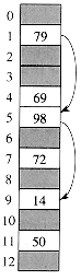
Figure 12.5 Insertion by double hashing. Here we have a
hash table of size 13 with h1(k) = k mod 13 and h2(k) = 1 + (k mod 11). Since 14
 1 mod 13 and 14 3 mod 11, the key 14 will be
inserted into empty slot 9, after slots 1 and 5 have been examined and found to
be already occupied.
1 mod 13 and 14 3 mod 11, the key 14 will be
inserted into empty slot 9, after slots 1 and 5 have been examined and found to
be already occupied.h1(k) = k mod m ,
h2(k) = 1 + (k mod m'),
(m2) probe
sequences are used, rather than (m), since each possible
(h1 (k), h2(k)) pair yields a
distinct probe sequence, and as we vary the key, the initial probe position
h1(k) and the offset h2(k) may
vary independently. As a result, the performance of double hashing appears to be
very close to the performance of the "ideal" scheme of uniform hashing.
Analysis of open-address hashing
of the hash table, as n and
m go to infinity. Recall that if n elements are stored in a table
with m slots, the average number of elements per slot is = n/m. Of course, with
open addressing, we have at most one element per slot, and thus n m, which implies 1.
h(k,
0), h(k, 1), . . . , h(k, m - 1) for each key k is equally
likely to be any permutation on 0, 1, . . . , m - 1. That is, each possible probe
sequence is equally likely to be used as the probe sequence for an insertion or
a search. Of course, a given key has a unique fixed probe sequence associated
with it; what is meant here is that, considering the probability distribution on
the space of keys and the operation of the hash function on the keys, each
possible probe sequence is equally likely.
= n/m < 1, the
expected number of probes in an unsuccessful search is at most 1/(1 - ), assuming uniform hashing.

(12.6)
 1? The probability that the first
probe accesses an occupied slot is n/m; thus,
1? The probability that the first
probe accesses an occupied slot is n/m; thus,

 n
/ m if n
m and j 0. After
n probes, all n occupied slots have been seen and will not be
probed again, and thus qi = 0 for i n.
< 1, the average number
of probes in an unsuccessful search is
n
/ m if n
m and j 0. After
n probes, all n occupied slots have been seen and will not be
probed again, and thus qi = 0 for i n.
< 1, the average number
of probes in an unsuccessful search is
(12.7)
a second probe is needed, with probability approximately 2 a third probe is
needed, and so on.
is a constant,
Theorem 12.5 predicts that an unsuccessful search runs in O(1) time. For
example, if the hash table is half full, the average number of probes in an
unsuccessful search is 1/(1 - .5) = 2. If it is 90 percent full, the average
number of probes is 1/(1 - .9) = 10.
requires at most 1/(1 - ) probes on average, assuming
uniform hashing.
< 1.
Inserting a key requires an unsuccessful search followed by placement of the key
in the first empty slot found. Thus, the expected number of probes is 1/(1 -
).
< 1, the expected number
of probes in a successful search is at most
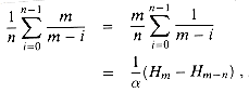
 is the ith harmonic number (as defined in equation (3.5)). Using the
bounds ln i
Hi ln
i + 1 from equations (3.11)and (3.12), we obtain
is the ith harmonic number (as defined in equation (3.5)). Using the
bounds ln i
Hi ln
i + 1 from equations (3.11)and (3.12), we obtain
Exercises
h(k, 0),
h(k, 1), . . . , h(k, m - 1) is a permutation of the slot
sequence 0, 1, . . . , m
- 1 if and only if
h2(k) is relatively prime to m. (Hint:
See Chapter 33.)
= 1/2. What is the
expected number of probes in an unsuccessful search? What is the expected number
of probes in a successful search? Repeat these calculations for the load factors
3/4 and 7/8.
e-n(n
- 1)/2m. (Hint: See equation (2.7).) Argue that when
n exceeds  , the
probability of avoiding collisions goes rapidly to zero.
, the
probability of avoiding collisions goes rapidly to zero.

(12.8)
 = 0.5772156649
. . . is known as Euler's constant and satisfies 0 < < 1. (See Knuth [121] for a
derivation.) How does this improved approximation for the harmonic series affect
the statement and proof of Theorem 12.7?
. Find the nonzero value for which the expected number of
probes in an unsuccessful search equals twice the expected number of probes in a
successful search. Use the estimate (1/) ln(1/(1 - )) for the number of probes
required for a successful search.
= 0.5772156649
. . . is known as Euler's constant and satisfies 0 < < 1. (See Knuth [121] for a
derivation.) How does this improved approximation for the harmonic series affect
the statement and proof of Theorem 12.7?
. Find the nonzero value for which the expected number of
probes in an unsuccessful search equals twice the expected number of probes in a
successful search. Use the estimate (1/) ln(1/(1 - )) for the number of probes
required for a successful search.
Problems
m/2. Open addressing is used
for collision resolution.
1/n2. Let the
random variable X = max1in Xi denote
the maximum number of probes required by any of the n insertions.
1/n.
 nQk.
nQk.
 h(k), and set
j 0.
(j +
l) mod m and i
(i + j) mod m, and return to step 2.
h(k), and set
j 0.
(j +
l) mod m and i
(i + j) mod m, and return to step 2.
 be a class of hash functions in which
each h maps the universe U of keys to {0, 1, . . . , m -
1}. We say that
be a class of hash functions in which
each h maps the universe U of keys to {0, 1, . . . , m -
1}. We say that  is
k-universal if, for every fixed sequence of k distinct keys
<x1, x2, . . . , xk>
and for any h chosen at random from
is
k-universal if, for every fixed sequence of k distinct keys
<x1, x2, . . . , xk>
and for any h chosen at random from  , the sequence
<h(xl), h(x2), . . . ,
h(xk)> is equally likely to be any of the
mk sequences of length k with elements drawn from {0,
1, . . . , m -1}.
, the sequence
<h(xl), h(x2), . . . ,
h(xk)> is equally likely to be any of the
mk sequences of length k with elements drawn from {0,
1, . . . , m -1}.
 is 2-universal, then it is universal.
 defined in Section 12.3.3 is not
2-universal.
defined in Section 12.3.3 is not
2-universal.
 in Section 12.3.3 so that each
function also contains a constant term b, that is, if we replace
h(x) with
in Section 12.3.3 so that each
function also contains a constant term b, that is, if we replace
h(x) with
ha, b(x)=a
x + b, is 2-universal.
Chapter notes